Polynomial of degree N
whit N from 2 to 20
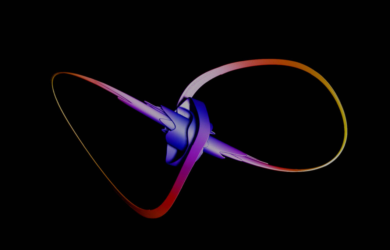
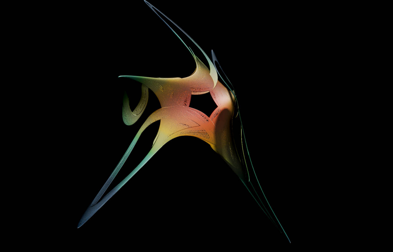
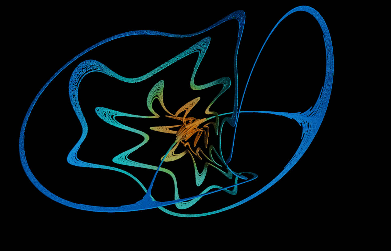
Polynom N-order with N = 11
Pn3D_o11_006a.sca
3D attractors are point clouds generate from sequences of numbers pn{xn,yn,zn} ⇒ pn ∈ R3, n ∈ N,
where n0→∞ denotes the step of the iteration process starting from a initial p0{x0,y0,z0} point.
In the cloud each next point is function of the previous one:
\[ \eqalign { x_{i+1} = \xi(x_i, y_i, z_i) & \\ y_{i+1} = \phi(x_i, y_i, z_i) & \\ z_{i+1} = \psi(x_i, y_i, z_i) & } \qquad \Bigg\{ \eqalign { & x, y, z \in R \\ & [0, i, n_{\rightarrow\infty}[ \text{ } \Rightarrow i,n \in N \\ } \]
In the computational code:
p(x,y,z) represent the i-th point pi{xi,yi,zi}
kj→m are constant values characteristic of any single attractor, where k ∈ R3 and [0,j,m] ⇒ j,m ∈ N
pNew ∈ R3 is the new point: pi+1{xi+1,yi+1,zi+1} that will calculated
In the ATTRACTORS window of glChAoS.P:
left side panel contains starting point coordinates p0{x0,y0,z0}
right side panel contains constant values used in the expression of the current attractor, where: kj{x,y,z} = k[j](x,y,z)
kj values can also be generated randomly between [min, kj, max] interval.
Colors are indicative of point speed: distance between pi and pi+1
This type of attractors are deeply described in the Julien C. Sprott book entitled: "Strange Attractors: Creating Patterns in Chaos"
The PDF version is accessible freely from author site: Strange Attractors: Creating Patterns in Chaos and
starting from chapter 4 he introduces the polynomial 3D attractor of order N
Briefly, below, I will describe the general formula that characterize the attractor (referring for further information to cited Julien C. Sprott book), and the universal formula personally developed to calculate any polynom of N order
Starting from the 2nd order polynomial, the simplest system of equations for this type of attractor, we get:
\[ \begin{align} x_{i+1} & = k_{0x} + k_{1x} \centerdot x_i + k_{2x} \centerdot y_i + k_{3x} \centerdot z_i + k_{4x} \centerdot x_i^2 + k_{5x} \centerdot x_i y_i + k_{6x} \centerdot x_i z_i + k_{7x} \centerdot y_i^2 + k_{8x} \centerdot y_i z_i + k_{9x} \centerdot z_i^2 \\ y_{i+1} & = k_{0y} + k_{1y} \centerdot x_i + k_{2y} \centerdot y_i + k_{3y} \centerdot z_i + k_{4y} \centerdot x_i^2 + k_{5y} \centerdot x_i y_i + k_{6y} \centerdot x_i z_i + k_{7y} \centerdot y_i^2 + k_{8y} \centerdot y_i z_i + k_{9y} \centerdot z_i^2 \\ z_{i+1} & = k_{0z} + k_{1z} \centerdot x_i + k_{2z} \centerdot y_i + k_{3z} \centerdot z_i + k_{4z} \centerdot x_i^2 + k_{5z} \centerdot x_i y_i + k_{6z} \centerdot x_i z_i + k_{7z} \centerdot y_i^2 + k_{8z} \centerdot y_i z_i + k_{9z} \centerdot z_i^2 \\ \end{align} \]
These equations have 10 coefficients for any variable: are 30 coefficients in total
Passing to 3rd order polynomial, only ONE superior degree, we have:
\[ \begin{align} x_{i+1} & = k_{0x} + k_{1x} \centerdot x_i + k_{2x} \centerdot y_i + k_{3x} \centerdot z_i + k_{4x} \centerdot x_i^2 + k_{5x} \centerdot x_i y_i + k_{6x} \centerdot x_i z_i + k_{7x} \centerdot y_i^2 + k_{8x} \centerdot y_i z_i + k_{9x} \centerdot z_i^2 + k_{10x} \centerdot x_i^3 + k_{11x} \centerdot x_i^2 y_i + k_{12x} \centerdot x_i^2 z_i + k_{13x} \centerdot x_i y_i^2 + k_{14x} \centerdot x_i y_i z_i + k_{15x} \centerdot x_i z_i^2 + k_{16x} \centerdot y_i^3 + k_{17x} \centerdot y_i^2 z_i + k_{18x} \centerdot y_i z^2 + k_{19x} \centerdot z_i^3 \\ y_{i+1} & = k_{0y} + k_{1y} \centerdot x_i + k_{2y} \centerdot y_i + k_{3y} \centerdot z_i + k_{4y} \centerdot x_i^2 + k_{5y} \centerdot x_i y_i + k_{6y} \centerdot x_i z_i + k_{7y} \centerdot y_i^2 + k_{8y} \centerdot y_i z_i + k_{9y} \centerdot z_i^2 + k_{10y} \centerdot x_i^3 + k_{11y} \centerdot x_i^2 y_i + k_{12y} \centerdot x_i^2 z_i + k_{13y} \centerdot x_i y_i^2 + k_{14y} \centerdot x_i y_i z_i + k_{15y} \centerdot x_i z_i^2 + k_{16y} \centerdot y_i^3 + k_{17y} \centerdot y_i^2 z_i + k_{18y} \centerdot y_i z^2 + k_{19y} \centerdot z_i^3 \\ z_{i+1} & = k_{0z} + k_{1z} \centerdot x_i + k_{2z} \centerdot y_i + k_{3z} \centerdot z_i + k_{4z} \centerdot x_i^2 + k_{5z} \centerdot x_i y_i + k_{6z} \centerdot x_i z_i + k_{7z} \centerdot y_i^2 + k_{8z} \centerdot y_i z_i + k_{9z} \centerdot z_i^2 + k_{10z} \centerdot x_i^3 + k_{11z} \centerdot x_i^2 y_i + k_{12z} \centerdot x_i^2 z_i + k_{13z} \centerdot x_i y_i^2 + k_{14z} \centerdot x_i y_i z_i + k_{15z} \centerdot x_i z_i^2 + k_{16z} \centerdot y_i^3 + k_{17z} \centerdot y_i^2 z_i + k_{18z} \centerdot y_i z^2 + k_{19z} \centerdot z_i^3 \\ \end{align} \]
Now these equations have 20 coefficients for any variable: 60 coefficients in total
And in general a nth order polynomial, with 3 components (3D), have:
\[ \eqalign { \text{ coefficients } \text{ } = \text{ } } \eqalign { ((n+1) \centerdot (n+2) \centerdot (n+3)) \above 1pt 2 } \quad \eqalign { \Rightarrow \quad n \in N } \]
So, for a 4th order (quartic) we'll have 105 coefficients, 5th (quintic) have 168 coefficients, and so on.
With glChAoS.P we can to calculate equations until the 20th order: are 5315 total coefficients (1771*3).
This is only a limit dictated by common sense, could go further, but the calculus becomes very slow, mostly the search for a "stable" attractor based on Lyapunov exponent (chapter2 of Julien C. Sprott book).
Below some examples of this type of attractors, with different degree n.
You can to start wglChAoS.P with a specific attractor directly from explore button.
Select lowResources for low resources devices (e.g. mobile devices)
|
Resolution:
X
render in new window
|
This second part si dedicated to computational code: the universal formula to calculate the equations for any n.
For simplicity we go back to the 2nd order equations (quadratic), we can write more verbosely:
\[ \begin{align} x_{i+1} & = k_{0x} + k_{1x} \centerdot x_i^1 + k_{2x} \centerdot y_i^1 + k_{3x} \centerdot z_i^1 + k_{4x} \centerdot x_i^2 + k_{5x} \centerdot x_i^1 y_i^1 + k_{6x} \centerdot x_i^1 z_i^1 + k_{7x} \centerdot y_i^2 + k_{8x} \centerdot y_i^1 z_i^1 + k_{9x} \centerdot z_i^2 \\ y_{i+1} & = k_{0y} + k_{1y} \centerdot x_i^1 + k_{2y} \centerdot y_i^1 + k_{3y} \centerdot z_i^1 + k_{4y} \centerdot x_i^2 + k_{5y} \centerdot x_i^1 y_i^1 + k_{6y} \centerdot x_i^1 z_i^1 + k_{7y} \centerdot y_i^2 + k_{8y} \centerdot y_i^1 z_i^1 + k_{9y} \centerdot z_i^2 \\ z_{i+1} & = k_{0z} + k_{1z} \centerdot x_i^1 + k_{2z} \centerdot y_i^1 + k_{3z} \centerdot z_i^1 + k_{4z} \centerdot x_i^2 + k_{5z} \centerdot x_i^1 y_i^1 + k_{6z} \centerdot x_i^1 z_i^1 + k_{7z} \centerdot y_i^2 + k_{8z} \centerdot y_i^1 z_i^1 + k_{9z} \centerdot z_i^2 \\ \end{align} \]
and more... remembering also that k0 = 1 we can write:
\[ \begin{align} x_{i+1} & = k_{0x} \centerdot x_i^0 y_i^0 z_i^0 + k_{1x} \centerdot x_i^1 y_i^0 z_i^0 + k_{2x} \centerdot x_i^0 y_i^1 z_i^0 + k_{3x} \centerdot x_i^0 y_i^0 z_i^1 + k_{4x} \centerdot x_i^2 y_i^0 z_i^0 + k_{5x} \centerdot x_i^1 y_i^1 z_i^0 + k_{6x} \centerdot x_i^1 y_i^0 z_i^1 + k_{7x} \centerdot x_i^0 y_i^2 z_i^0 + k_{8x} \centerdot x_i^0 y_i^1 z_i^1 + k_{9x} \centerdot x_i^0 y_i^0 z_i^2 \\ y_{i+1} & = k_{0y} \centerdot x_i^0 y_i^0 z_i^0 + k_{1y} \centerdot x_i^1 y_i^0 z_i^0 + k_{2y} \centerdot x_i^0 y_i^1 z_i^0 + k_{3y} \centerdot x_i^0 y_i^0 z_i^1 + k_{4y} \centerdot x_i^2 y_i^0 z_i^0 + k_{5y} \centerdot x_i^1 y_i^1 z_i^0 + k_{6y} \centerdot x_i^1 y_i^0 z_i^1 + k_{7y} \centerdot x_i^0 y_i^2 z_i^0 + k_{8y} \centerdot x_i^0 y_i^1 z_i^1 + k_{9y} \centerdot x_i^0 y_i^0 z_i^2 \\ z_{i+1} & = k_{0z} \centerdot x_i^0 y_i^0 z_i^0 + k_{1z} \centerdot x_i^1 y_i^0 z_i^0 + k_{2z} \centerdot x_i^0 y_i^1 z_i^0 + k_{3z} \centerdot x_i^0 y_i^0 z_i^1 + k_{4z} \centerdot x_i^2 y_i^0 z_i^0 + k_{5z} \centerdot x_i^1 y_i^1 z_i^0 + k_{6z} \centerdot x_i^1 y_i^0 z_i^1 + k_{7z} \centerdot x_i^0 y_i^2 z_i^0 + k_{8z} \centerdot x_i^0 y_i^1 z_i^1 + k_{9z} \centerdot x_i^0 y_i^0 z_i^2 \\ \end{align} \]
now passing to computational code, if we set:
    float cf[10];
    cf[0] = x^0 * y^0 * z^0;
    cf[1] = x^1 * y^0 * z^0;
    cf[2] = x^0 * y^1 * z^0;
    ...
    cf[9] = x^0 * y^0 * z^2;
and using vectors k[i](x,y,x) instead of {kix, kiy, kiz}, finally we can calculate the new point Pn+1 as summation of K * cf:
    vec3 pNew = vec3(0.0, 0.0, 0.0);
    for(int i; i<10; i++)
        pNew += k[i] * cf[i];
At this point we need only to calculate dynamically the values of cf[0], cf[1], cf[2] ... etc.
So, we consider the degree of the polynomial (this case 2) and we calculate, for any variable (x, y, z), any power with exponents 0, 1 and 2.
    const int order = 2;
    float ex[order+1], ey[order+1], ez[order+1];

    ex[0] = ey[0] = ez[0] = 1.f; // x[0]=1 as x^0
    for(int i=1; i<=order; i++) {
        ex[i] = ex[i-1] * x;
        ey[i] = ey[i-1] * y;
        ez[i] = ez[i-1] * z;
    }
    // x[1] = x[0] * x = 1 * x --> x^1
    // and
    // x[2] = x[0] * x [1] * x --> x^2
usng also here the vectors, we rewrite the previous loop, with p(x,y,z) actual point:
    const int order = 2;
    static vec3 elv[order+1];

    elv[0] = vec3(1.f);
    for(int i=1; i<=order; i++)
        elv[i] = elv[i-1] * p;
and now we calculate the cf coefficients, dynamically... making sure that the sum of the exponents does not exceed the degree of the polynomial:
    int j = 0;
    // I use reverse loop because test on 0 is faster
    for(int x=order-1; x>=0; x--)
        for(int y=order-1; y>=0; y--)
            for(int z=order-1; z>=0; z--)
                if(x+y+z <= order)
                    cf[j++] = elv[x].x * elv[y].y * elv[z].z;

    // and now x^2*y^0*z^0... y^2, z^2 separately
    cf[j++] = elv[order].x;
    cf[j++] = elv[order].y;
    cf[j++] = elv[order].z;
so we arrived at the summation seen above
        int nCoeff = j;
        vec3 pNew = vec3(0.0, 0.0, 0.0);

        for(int i=0; i < nCoeff; i++) pNew += k[i] * cf[i];
the total number of coefficients can be calculate also from formula, previously seen:
nCoeff = ((order+1) * (order+2) * (order+3) / 2) / 3; .. (because we are using vectors of 3 components)
Now we write the whole formula, valid for any "order" of polynomial, so we can calculate also an degree of 20!, with 1771*3 = 5313 coefficients.
    // input : p, current (x,y,z) point
    // output: pNew, next calculate point
    void PowerN3D(vec3 &p, vec3 &pNew)
    {
        const int order = N; // where N is any int number
        vec3 elv[order+1];

        elv[0] = vec3(1.f);
        for(int i=1; i<=order; i++)
            elv[i] = elv[i-1] * p;

        int j = 0;
        // reverse index, only because compare with 0 is faster
        for(int x=order-1; x>=0; x--)
            for(int y=order-1; y>=0; y--)
                for(int z=order-1; z>=0; z--)
                    if(x+y+z <= order)
                        cf[j++] = elv[x].x * elv[y].y * elv[z].z;

        cf[j++] = elv[order].x;
        cf[j++] = elv[order].y;
        cf[j++] = elv[order].z;

        int nCoeff = j;
        pNew = vec3(0.f);

        for(int i=0; i < nCoeff; i++) pNew += kVal[i] * cf[i];
    }
This is a demonstrative function: need to declare and alloc cf
The source code is slightly different: I used std::vector, iterators and pointers, instead of static array, and it's a little more cryptic for those who do not use the C ++ language:
    void PowerN3D::Step(vec3 &p, vec3 &pNew)
    {
        elv[0] = vec3(1.f);
        for(int i=1; i<=order; i++) elv[i] = elv[i-1] * p;

        auto itCf = cf.begin();
        for(int x=order-1; x>=0; x--)
            for(int y=order-1; y>=0; y--)
                for(int z=order-1; z>=0; z--)
                    if(x+y+z <= order) *itCf++ = elv[x].x * elv[y].y * elv[z].z;

        *itCf++ = elv[order].x;
        *itCf++ = elv[order].y;
        *itCf++ = elv[order].z;

        pNew = vec3(0.f);

        itCf = cf.begin();
        for(auto &it : kVal) pNew += it * *itCf++;
    }